插值和空间分析(二)_变异函数分析(R语言)
方法1、散点图
hscat(log(zinc)~1, meuse, (0:9)*100)

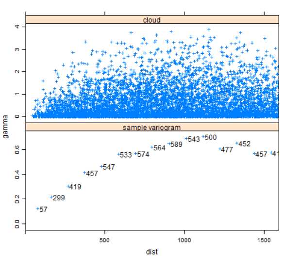
方法2、变异函数云图
library(gstat)
cld <- variogram(log(zinc) ~ 1, meuse, cloud = TRUE)
svgm <- variogram(log(zinc) ~ 1, meuse)
d <- data.frame(gamma = c(cld$gamma, svgm$gamma),
    dist = c(cld$dist, svgm$dist),
    id = c(rep("cloud", nrow(cld)), rep("sample variogram", nrow(svgm)))
    )
xyplot(gamma ~ dist | id, d,
    scales = list(y = list(relation = "free",
      #ylim = list(NULL, c(-.005,0.7)))),
      limits = list(NULL, c(-.005,0.7)))),
    layout = c(1, 2), as.table = TRUE,
    panel = function(x,y, ...) {
        if (panel.number() == 2)
            ltext(x+10, y, svgm$np, adj = c(0,0.5)) #$
        panel.xyplot(x,y,...)
    },
    xlim = c(0, 1590),
    cex = .5, pch = 3
)
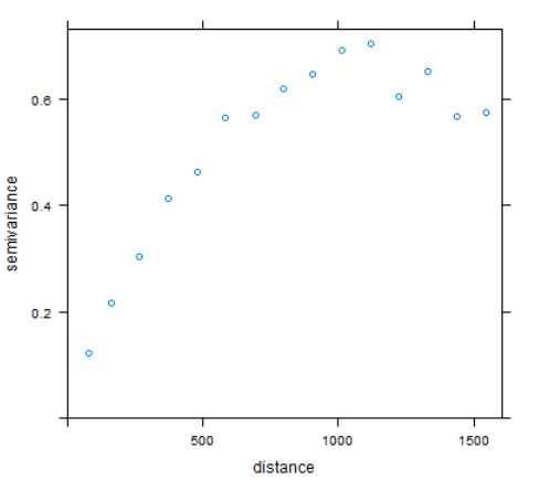
plot(variogram(log(zinc) ~ 1, meuse)) // 对每一个距离去平均
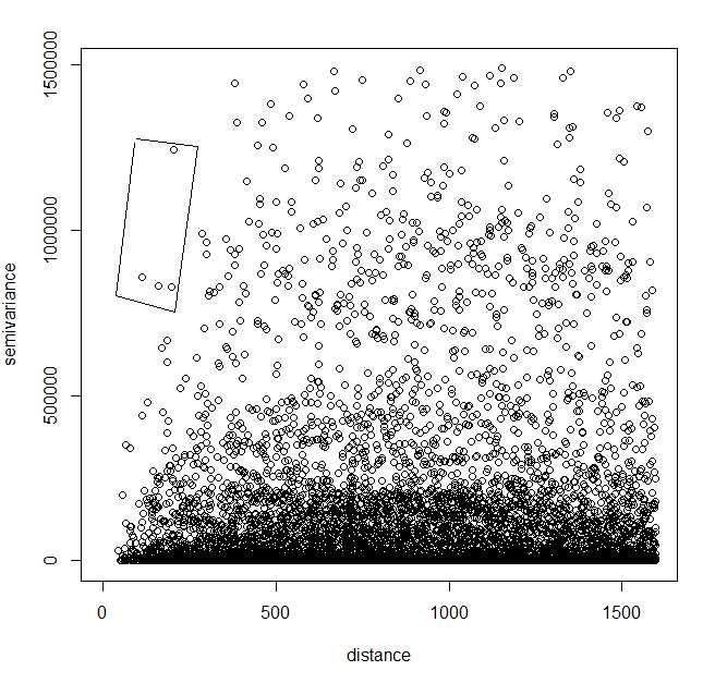
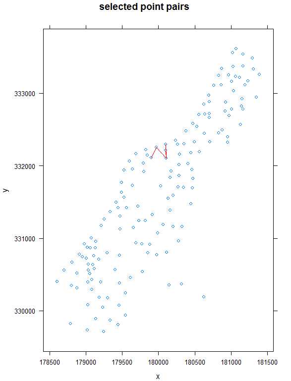
sel <- plot(variogram(zinc ~ 1, meuse, cloud = TRUE), digitize = TRUE)
plot(sel, meuse)
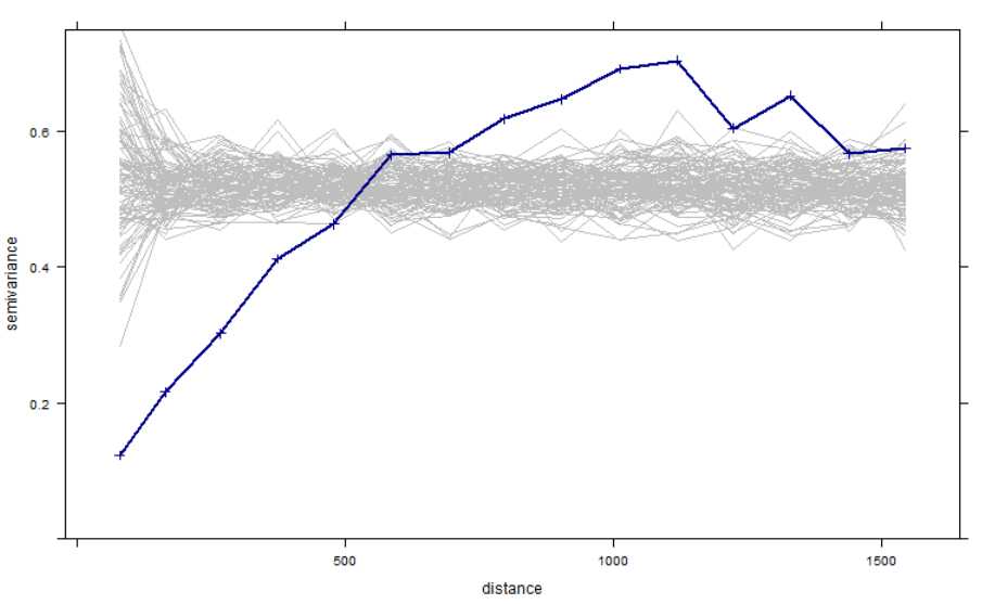
v <- variogram(log(zinc) ~ 1, meuse)
print(xyplot(gamma ~ dist, v, pch = 3, type = ‘b‘, lwd = 2, col = ‘darkblue‘,
    panel = function(x, y, ...) {
        for (i in 1:100) {
            meuse$random = sample(meuse$zinc)
            v = variogram(log(random) ~ 1, meuse)
            llines(v$dist, v$gamma, col = ‘grey‘)
        }
        panel.xyplot(x, y, ...)
    },
    ylim = c(0, 0.75), xlab = ‘distance‘, ylab = ‘semivariance‘
))
文章来自:http://www.cnblogs.com/takeaction/p/4123296.html